For whom the bell-curve tolls

As I mentioned in my previous post on measures of central tendency, this is part 2 of a 3-part post on some basic statistical concepts.
If you’ve ever been graded on a curve or have heard the term “bell curve”, then you know a bit about the normal distribution. This post will focus on the concept of the normal distribution and some very basic elements around it. Although this concept might seem fairly straightforward, there is a lot of detail and math that goes into it, which I will not be going into here. Also, the normal distribution is only one of MANY distributions, which I also won’t cover.
Why am I focusing on the normal distribution? This answer comes in two parts:
- Why use any probability distribution? Because they help make decisions. We use probability distributions to graph all the possible outcomes of an event and the probabilities for each of those outcomes occurring so we can determine the likelihood of something happening. These probabilities and the shape of their distribution gives us a decision making framework.
- Since there are so many other distributions, what makes the normal distribution so special? Basically, it is due to something called the Central Limit Theorem which results in a lot of events in the world roughly looking like a normal distribution curve when graphed including height, weight, IQ, and even shoe size (go figure!).
Here is a really fun way of looking at why it works using a device called the Galton Board. See how the beans seem to come in randomly but with enough beans they naturally trend towards a normal distribution? That’s pretty much the idea.
If a probability distribution provides a decision making framework, then the normal distribution would be the most common of those frameworks.
First things first, we need to discuss the difference between a frequency distribution and a probability distribution. I am going to focus on the normal distribution as a probability distribution but you should know how to graph data as a frequency distribution to understand how the probability distribution is determined.
Frequency Distribution
A frequency distribution takes the actual occurrence of an event and graphs the number of times each value for that event is seen; a frequency distribution is about describing a data set. Exam grades are a good example. If you have an exam out of 20 marks and 350 students in the class, you will get a lot of overlap in grades. With only 21 possible outcomes (0 out of 20 as the lowest and 20 out of 20 as the highest) but with 350 students you might get a simple bar chart that looks something like this:
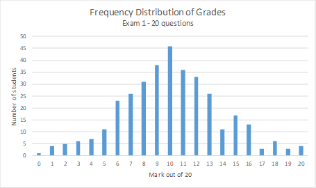
As can be seen, around 46 students received the mark of 10 out of 20, which is also the most common grade. This makes 10 out of 20 both the median and mode for this data set. The mean (when rounded to a whole number) is also 10 out of 20. The number – or frequency – of students receiving marks OTHER than 10 out of 20 were all lower.
Although the graph is somewhat bell-shaped – like the normal distribution curve – this is still a frequency distribution in that it takes the exam marks of students and counts them. If I asked what the probability was of a student getting 17 out of 20 the next time you give this same exam to a different class, this graph (in its current form) could not answer that question. It can only tell me how many students actually received a mark of 17 out of 20 (3 in this case) on this exam. A frequency distribution can tell a nice story about something that has already happened but it can’t (yet) help predict what will happen in the future. This is where the normal probability distribution can help.
Normal (Probability) Distribution
The normal distribution curve is a continuous probability curve. The continuous part means that – unlike the frequency distribution above – the normal curve can take on any value under the curve. The probability part means you can use the distribution to estimate the chance or likelihood of any event on that curve. So, you could ask how many people would have scores between 9.25 and 15.5 (if part marks exist) the next time you gave this exam. In theory, you could also determine how many people would have scores between 9.273 and 15.568, which is where the continuous part comes in.
In the case of exam marks it might not seem that useful to use continuous data, but the ability to determine probability for continuous data becomes more helpful for things like medicine dosages, height, or weight but you get the idea.
This is what the graph above for Exam 1 looks like when you overlay a normal distribution curve:
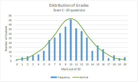
As can be seen, there are some marks in the frequency distribution that would be above or below the normal curve but the frequency distribution looks pretty close to the normal curve.
Properties of the Normal Distribution Curve
Now, about the normal distribution curve. What are its properties?
- The data is symmetrical around the mean (or average), In the example above, the mean is 10.08 (to 2 decimal places) so around 10 out of 20 if you’re rounding to a whole number. “Symmetrical” says that 50% of the marks are below the mean (of 10) and 50% of the marks are above the mean.
- The total area under the curve equals 100% of possible values. But really, that just makes sense if 50% is above the mean and 50% is below because 50% + 50% = 100%
- The mean = median = mode. (If you need a refresher on what these measures are, please refer to my last post here). This is pretty clear in the graph above but it always is when you structure the data to prove a point. 😉
In order to determine the shape of a probability curve, there are only 2 parameters: the mean (or average) and the standard deviation.
The mean is the peak of the curve while the standard deviation determines the spread of the data, or how far away from the mean the data tends to fall.
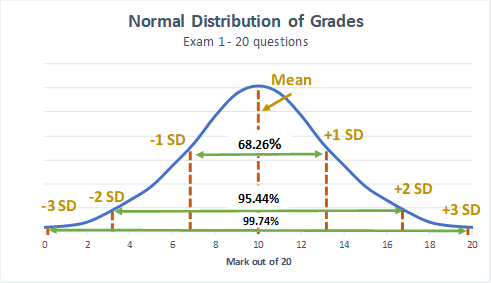
The cool thing about the standard deviation is that it determines the shape of the curve. The other thing is that 99.7% of the probabilities fall within 3 standard deviations of the mean. But let’s talk about the latter first.
So, because the normal distribution is symmetrical, the 3 standard deviations to the left of the mean are 49.87% of the data and the 3 standard deviations to the right of the mean are also 49.87% of the data which means that, as mentioned above, 99.7% of the data is within 3 standard deviations. However, each standard deviation IS NOT created equal. This is how it actually works:
- +/- 1 standard deviation = 68.26%
- +/- 2 standard deviations = 95.44%
- +/- 3 standard deviations = 99.74%
Using the grades example above for Exam 1, visually this means (note that SD = standard deviation in the graph):
An example of how the normal distribution curve could be used in real life draws on the shoe size example I mentioned at the beginning of the post. Think about the last time you went shoe shopping. Let’s say shoe size is normally distributed and the average shoe size for women is 8 with a standard deviation of 1. If Nike knows this, they would likely make most of their shoes between sizes 6 and 10 (2 standard deviations from the mean or 95% of the area under the curve) because they will sell most of their shoes in this size range. If you were a size 5 or 11 you would probably not see too many of these sizes on the shelves because fewer women wear these sizes and it would be less profitable for Nike to make too many of them.
Of course, there are some challenges to the data as there often is. Real life data – such as the grades example I’ve been using – is very rarely perfectly normally distributed. So, what happens when your data is not perfect and some rules seem to get broken (as will happen more times than not)?
In the Exam 1 grades example I’ve been using, I made the chart look as though the 3 standard deviations stay within the range of marks 0 – 20; however, this is often not the case and there are a few challenges when the standard deviations go into negative territory or above the maximum possible score.
Issue #1
The way the graph above looks, 99.74% of grades fall between 0.5 and 19.5 out of 20 with anything in between being possible. How likely is it for someone to get 12.37 out of 20 on the exam? Unless there is a way to grade each question out of 100 to get down to a score of 2 decimal places, the most you’d expect is maybe quarter or half marks. As a result, trying to calculate the probability on a continuous scale may not make the most intuitive sense for this particular type of data. But that doesn’t mean it’s wrong, it just means it’s a bit harder to interpret.
Issue #2
More importantly, the graph does not actually show the REAL standard deviation of the data. I adjusted it a bit to make a simple point tied up with a nice bow. In fact, the mean was 10.08 and the standard deviation was 3.77 (rounded). If I was to calculate the standard deviations, then:
+3 standard deviations is actually 10.08 + (3 * 3.77) = 21.39 and
-3 standard deviations is actually 10.08 – (3 * 3.77) = -1.23.
Let’s say bonus marks were available and getting 21.39 out of 20 is actually possible (notwithstanding my issue in the first point above), it’s actually not likely that a score of -1.23 is possible without deducting marks for wrong answers, which is unusual on most exams.
What to do?
As a result, this variability (going below zero) does not make sense in the context of the data and while the data follows some of the rules of normal distribution, it is not perfect. What should be done in these cases? Well, there are a couple things that are fairly common:
- In many cases, the standard error is used instead of standard deviation because it’s less likely to get negative values. In a 2011 article published by NCBI they state that by using standard error “the intervals obtained, compared to the mean value, are shorter, thus hiding the skewed nature of the data.”
- Other times, the data may need to be transformed to make the distribution more closely match that of the normal distribution. By far the most common type of transformation is logarithmic.
But now I’m getting into too much detail for one post and this really does require a deeper knowledge of statistics so I will leave it at this: if the distribution doesn’t make sense, dig deeper to understand why (and be open to learning how to fix it).
Standard Normal Distribution
Another thing I wanted to briefly mention is the standard normal distribution. This is a special case of the normal distribution when the mean is 0 and the standard deviation is +/- 1 and it is sometimes called the Z distribution. Any value on the normal distribution can be converted to a Z distribution by using the z-score formula, which I will discuss in the next post. Why would you want to convert a normal distribution to a Z distribution? So you can compare the distributions of different data. For example, you might want to know what product price is better so you do a test of two different prices. However, the two tests have different mean (average) prices. By converting to standard normal distributions you can put the data in similar terms, not unlike finding the common denominator in fractions, so you can do an apples to apples comparison.
“Flattening the Curve“
I can’t really finish this post and discussion about the normal curve without at least touching on the subject of “flattening the curve”. That phrase has become so commonplace in the last few weeks that anyone reading this now will not really need me to say that it refers to social distancing and self-isolation as it relates to the COVID-19 pandemic. So, given the explanation of the normal distribution curve, how does this relate and/or explain the concept of “flattening the curve”?
Before I begin, I’d like to go over some caveats:
- The graph everyone has seen on TV and in the media is being used to describe a complex ecosystem and epidemiological phenomenon in as simple a way as possible. Similar to my Exam 1 grades example above, the curve cannot go into below zero territory as that does not make sense but yet the math might actually allow that so transformations or other accommodations might need to be done.
- As we’ve heard about the Spanish Flu of 1918, there were multiple waves where the infection rates dropped then surged again, which suggests not one nice bell curve but a curve with multiple humps.
- Epidemiological curves tend to have longer tails before they get to zero, which would result in a skewed distribution.
If you are seriously interested in epidemiology and you’d like to learn more, here is a link to the CDC website that provides the contents of an Intro to Epidemiology textbook.
The image below with the two normal distribution curves has become common in the media in the last month. Take a look at the left half of either bell curve; it looks like an exponential growth curve, doesn’t it? Hence, all the talk about exponential growth in COVID-19. When the media talks about the peak of the virus, they are talking about the time when we hit the highest number of daily cases – or where the mean = median = mode on the normal distribution – before cases start going down. I should note that we will not know we have hit that peak or where that mean = median = mode will be until we start seeing the decline. Up to this point, only a few countries believe they have seen the “other side of the mountain” and others are hoping for it to come quickly – but not too quickly – so we can start seeing the decline.
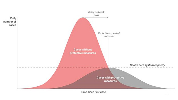
Image taken from medscape website
As previously discussed, the mean is the peak of the curve and the standard deviation is what determines the shape, or spread, of the curve. If you look at the red curve, you will see that the peak (or mean daily cases) is high and the spread (or standard deviation) is narrow. What this says is that without protective measures, the exponential growth will be quick but the peak will also come quickly before the decline starts. So, why would we want to flatten the curve – seen in grey below – if it takes so much longer to get to the peak and that much longer to get to the end of the pandemic?
There are actually several answers to this but the graph is basically illustrating it is because the capacity of our health care systems can’t handle the load if we let the red chart happen. Yes, the virus will spread faster and likely be done faster if we do nothing but it’s the cost of what that means that we can’t see in this graph. Remember, statistics can help show the trends in data but we still need to interpret what that means in life.
The interpretation is that hospitals will be over capacity so really sick people may not be able to get help, which will result in more deaths. So, if we are able to spread out the number of daily cases, it will take longer to get to the other side of the mountain but the hope is that hospitals can cope with the rise in patients so fewer people will die.
By lowering the mean daily cases and widening the standard deviation, another hope is that we reduce the overall percent of the population that gets infected because maybe it gives us more time to find a vaccine and we don’t have to rely on herd immunity to kick in. Fewer infections also means fewer deaths. That is the math – and some of the interpretation – behind these graphs anyway. Since we have not yet seen the peak (in North America anyway) – although we do have historical data and data from other countries to help us model what it might look like – we are hoping this is what will happen.
Another argument I hear frequently is how do we know if social distancing or self-isolation is working? Of course we will never know for certain what the curve would have looked like if we did nothing – this is only something science fiction and theories of parallel universes could possibly answer – but our modeling and projections can give us pretty good ideas of how we would have fared if we chose to do nothing.
Anyway, this is the basic introduction to normal distribution and a couple examples of how it can be used or how it is being interpreted. In my next post, I will tackle the concept of statistical testing and how it is used (primarily in a business context).
Finally, if you find the concept of probabilities and distributions interesting, and if you haven’t already done so, I highly recommend taking some statistics courses or reading some books on the subject to familiarize yourself with them and their uses. I also really like this blog and there is some good basic info on the 6 Common Probability Distributions.