Pretty little spreadsheets

Most people who have worked in an organization have, at one time or another, come across a spreadsheet. Perhaps you have been the author or merely a recipient, but spreadsheets are still a fairly common way to share data, information, or charts. Whether you are a Google Sheets or Microsoft Excel person, it is important to consider how your spreadsheet is formatted. If a spreadsheet is being shared, the formatting should also consider what the focus of the content is and how to structure the information to best convey this message.
Here’s an example of a very common type of spreadsheet. It contains sales information for stores within a chain or in which a particular organization sells product. The data is a mix of both words and numbers, including calculations. In this case, the “total rev” column is a sum of the “rev” and “misc rev” columns. Also note the numbers are not all of the same type as there are store numbers, unit sales, and currency revenues.
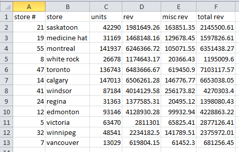
What makes this spreadsheet, let’s be honest, pretty ugly? Some of you copy people out there might say improper use or lack of capitalization. Or what about the inconsistent word contractions? Others might say the unit and revenue numbers are hard to read. Or, you might think the mix of left and right justification to be visually, well, yucky. In my opinion, you would all be correct. This spreadsheet has several challenges and could be fixed in a few simple formatting steps that would only take minutes to do in Excel.
So, here are some steps I would take to turn this information into a pretty little spreadsheet and help the reader focus on the message being conveyed instead of getting lost in the ugliness of the formatting. Although I am using Microsoft Excel, most of these steps would work in Google Sheets as well.
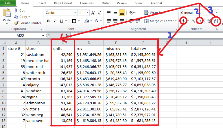
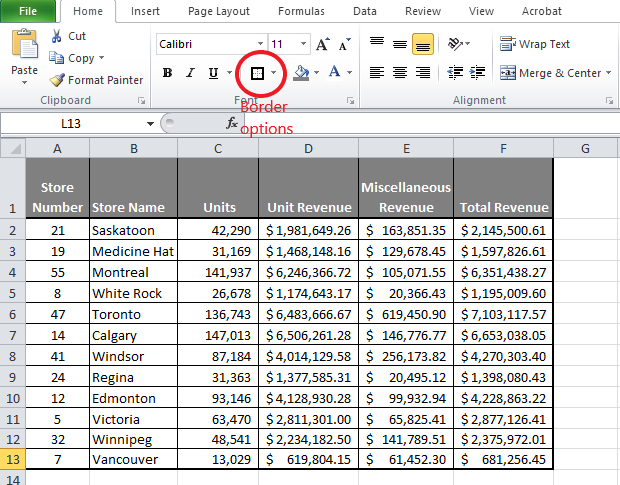
Step 1: Make the numbers easier to read and consistent with their type. The first thing I would do is change the revenue columns to the currency being used. I primarily work in dollars so I use that symbol. To do this, I would highlight columns D, E, and F altogether in the sample data above and click on the $ symbol. This will convert all those numbers to dollars (Number 1 in the diagram below).
Next, I would highlight column C and click on the comma symbol (Number 2 in the diagram below) then twice on the decrease decimal symbol, since units should be integers (Number 3 in the diagram below).
Already, you can see the numbers are a bit easier to read.
NOTE: You may also need to highlight all 4 of these columns after you format and widen the columns so the new formatting will fit properly. When I widen several columns at once, I highlight them altogether then go up to the column letters until the cursor turns into a cross symbol and left double click with the mouse. This automatically widens all highlighted columns to the correct size.
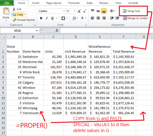
Step 2: Make the words look a bit prettier and more consistent. After formatting the numbers, I would change the data in the column called “store” to use proper capitalization. In Excel, there is a function called PROPER(). What this does is change the words to proper case, which just means the first letter of every word is capitalized. Unfortunately, you couldn’t do this directly in column B or you would overwrite the values. What you can do is go to column G and in cell G2 type =PROPER(B2) and “saskatoon” becomes “Saskatoon”. You can then drag this formula down all the way to G13 (or propagate the formula) and it will change all the values shown in B2 to B13 to proper case. You then COPY G2:G13 and use PASTE SPECIAL – VALUES into B2:B13. All the city names are now in proper case. Just don’t forget to delete the temporary formulae in column G since you only did a COPY not a CUT to move the city names.
For those of you who don’t like to see partial words, unclear heading titles, or words represented by symbols (ex. “misc rev” or “store #”), you could go ahead and change these now too. These would be manual typing changes though (or you could do an Edit – Replace if there are many similar contractions, like “rev” in the sample data). And I would also recommend doing a wrap text across all of Row 1 so the words don’t take up more room than the numbers. See the diagram below.
Step 3: Alignment and formatting for column headers. This step (and the next one) will probably have differing opinions. I generally prefer centering my column titles over the data with only one exception. The exception is when the data itself should either be left or right justified. In these cases, I tend to keep the title justified in the same way as the data. In the sample data, the data in the Store Name column is left justified so I keep the column title left justified.
For Store Number, I center BOTH the header and the data. If the store numbers were larger (say, 5 digits or more), I would probably left justify the column title and the data below.
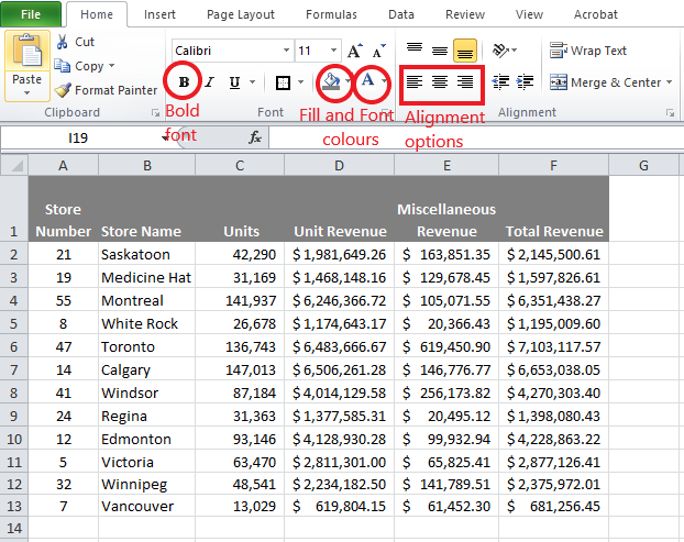
Another thing I like to do with my column titles is to make them stand out in some way. Some people might choose to bold the words or colour the cells. I like to change the fill colour of the cell to a dark grey and then change the font colour of the cell to white and bold it. This adds a nice contrast to the rest of the data and makes the titles stand out a bit.
Step 4: Cell borders. Another formatting element I like to use outside of simply number consistency within cells is the use of cell border lines to create some definition in how the numbers are viewed. It’s obvious in the sample data I’m using that this data is best suited to a tabular format. As a result, I like to make it look more like a table so the numbers don’t blend too much into each other. I like to use a “thick box border” for the title row and overall table and “all borders” for the interior cells. This is especially useful if you decide to print the table or to paste a screenshot of it in an email or internal memo. Please see Step 6 for the importance of print formatting.
You could in theory leave the table like this and it would look so much better than the original format. Nevertheless, there are a couple extra things about the formatting that would make the data not only flow better but also, make it easier for other people to quickly find key information in the data being shared.
Step 5: Sorting and Totals. Although the table after Step 4 hasn’t changed the order of the data or added any additional information, sometimes the data is easier to read or quickly get to the key points by incorporating these elements.
First, let’s talk about sorting the data. It’s clear the sample data I’ve used is discussing stores within a chain or organization. Would it make sense to sort it by store number or maybe alphabetically by store (city) name so people reading the data could quickly find the store in which they are most interested? Or maybe it would make more sense to sort it in descending order by units or revenue? The way it’s sorted would be business-specific but it’s an important point to consider. The way the sample data is currently sorted is very disorganized and it wastes time and reduces the focus because the audience cannot hone in on the most important piece(s) of information.
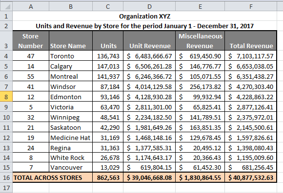
In addition to sorting data, adding some kind of total row or column can be useful as a snapshot of how the business is doing overall. If the sample data is a representation of all stores in the network or district, it seems like a pretty helpful piece of information to know the total units or total revenue for all stores not just within a store. I also like to do a subtle fill colour on the total row to make it stand out a bit.
And while I’m at it, a title should really be given to the table, which shows the organization name and time frame being represented by the data.
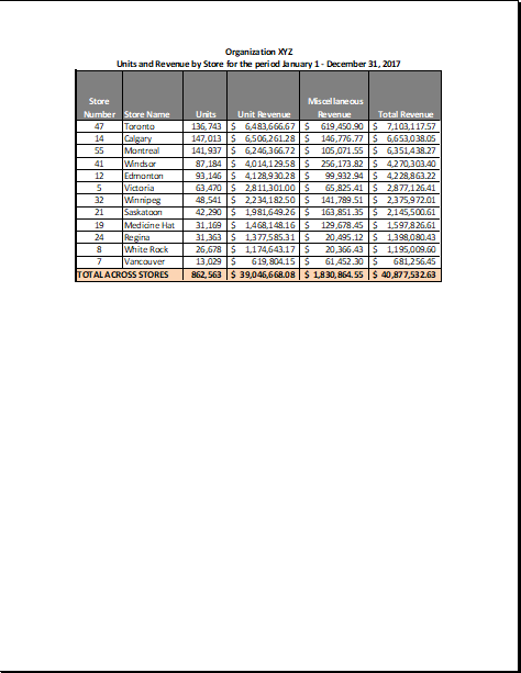
So here’s what I would do to the sample data to make it a bit more relevant, sorted by Total Revenue in this case.
Now let’s see what this looks like side by side with the original data:
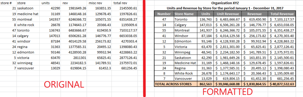
I don’t know about you, but in what took about 5 minutes of extra time, I think the data looks a lot more presentable. And even if it’s for my eyes only, it’s easier to quickly see the relevant information and what the focus of the data is. For example, I can easily see that most major cities in Canada have high revenue but Vancouver has the lowest. Formatting the data and sorting by total revenue let me quickly zero in on this anomaly. Now I can spend my time digging into why Vancouver might be under-performing.
In my next post, I will discuss no matter how great a table of data might be formatted, providing visual elements to consumers of your data is even better.
The last step I will discuss is what to do when you need to share your data in a hard copy format.
Step 6: Printing data. This is how your original data would look if you decided to print it out on paper and share it with your colleagues:
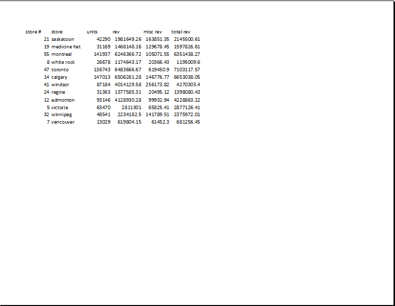
I’m not sure about you, but I’ve been to meetings where someone gave me this handout and I had to take a loooong drink of water and hold my tongue to prevent myself from lecturing my colleague on how to present data. It’s one thing to get a soft copy of a spreadsheet that looks like this; after all, I can play with it and look for things on my own. It’s another thing to get this information in printed form where I need to bring my ruler and calculator to a meeting just to understand what’s going on. And trust me, I’ve been to these types of meetings.
So, taking the formatted spreadsheet shown in steps 1 through 5, I do a few more things in Excel to make the printout look like this instead:
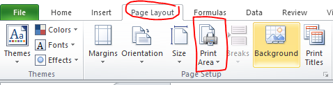
What did I do? First, I highlighted ONLY the area I want to print. So, if you have some random calculations hidden in other cells, they don’t make it into your printout. Once the area is highlighted, go to Page Layout –> Print Area and select Set Print Area from the drop down. This now tells the program to print ONLY the area highlighted.
After this, go to that little down arrow in the bottom right of the Page Setup ribbon. You can see it just in the bottom right of the image above. A pop up screen will appear that looks like this:
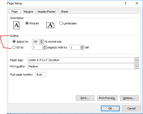
Here, scaling is important. If you have a lot of data – much more than I have in the sample data – you may want to select the “Fit to” option so you don’t get that one column or row on Page 2. However, make sure that if you use this option, the scale doesn’t get so small that the reader needs a magnifying glass to read the information.
The other thing I like to do is go to the “Margins” tab and go down to the bottom of the screen and click on “Horizontally” under the Center on page option.
If you have multiple pages and you want the same row or column to repeat at the top or side of each page, then you can select this option on the “Sheet” tab. I use this one occasionally but it’s not necessary for the sample data.
If you have data in multiple sections on the same sheet in a spreadsheet PLEASE make sure you format each section separately. And for goodness sake DO NOT try to print everything on one page so it looks like an eye chart. I’ve seen this happen time and again and it’s super distracting and annoying. It’s better to keep the different sections on separate pages to both focus the conversation and to make the data readable.
So, to turn data into pretty little spreadsheets is something I feel is super important and really only takes a few extra minutes and steps to do but has a powerful impact. It is one of the worst mistakes to lose your audience at the beginning of a meeting and spend the next 30-60 minutes trying to decipher data.
Well presented data should be used as a tool to further a discussion on strategy or to help solve a problem rather than becoming the focus of the meeting. If people are questioning what your spreadsheet is saying, you’ve already lost your audience and the point of your meeting. Now, if the audience trying to change the meaning of the data because they don’t like what it’s saying, that’s a post for another day. 🙂