A Tale of Two Tests

In my last two posts, I introduced measures of central tendency and the normal distribution. Why? Mostly because they are important statistical concepts but also because they lead nicely into the topic of statistical testing.
Statistical testing is very important because it provides a level of confidence providing that results from experiments are not due to chance or luck (good or bad). There are at least 4 key steps to perform in statistical testing. I say at least because for some of these you could easily break them down into smaller steps. Oftentimes, these are implied or done so seamlessly that it doesn’t seem like they are steps at all but trust me, they are. Each step will be discussed in turn but they are:
- Create a hypothesis
- Select the appropriate statistical test
- Determine the test statistic for your hypothesis
- Determine if the hypothesis should be rejected (statistically significant) or not rejected (statistically insignificant)
Just a note here, I will not be going into detail behind the math of these. My goal is to explain the concepts behind statistical testing and provide two examples of their use.
CREATE A HYPOTHESIS
You can’t go into an experiment or test without some idea of what you might get out of it. Imagine if a pharmaceutical company said, “Hey, let’s test this drug randomly and see if it cures something”. Right, sign me up for that? So, the first thing you want to do is come up with a hypothesis.
A hypothesis might be something as simple as we think a blue “Buy Now” button will convert more people than our current green “Buy Now” button. You would then day the null hypothesis is that the conversion of the blue button is higher and the alternate hypothesis is that the conversion of the control (or green) button is higher. The null hypothesis is what you are testing (or hypothesizing) and the alternate hypothesis is generally everything else.
Other hypothesis examples might be:
- Average customer satisfaction with support agents is at least 75%
- Ad A will perform better than Ad B on Facebook
- Retention rate of customers is at least 85%
- By putting product A at the beginning of the product page, conversion will be higher for ANY product.
- More males than females are buying product B
One important thing to note is that you can always reject the null hypothesis but you generally do not “accept” it; you just do not reject it. What’s the difference between accepting and not rejecting you ask? It’s because we can never definitively prove that the null is completely correct so we can never truly accept it. I read a courtroom analogy that I will borrow from here.
A jury cannot convict a defendant if there is reasonable doubt. Does the jury know for sure that the defendant is innocent? No. It returns the verdict of “not guilty”, which is not exactly the same as innocent. It’s similar for hypothesis testing. We will never know for sure if the null hypothesis is actually true so we can simply not reject it.

SELECT THE APPROPRIATE STATISTICAL TEST
Not all tests are created equal. There are specific tests depending on:
- the type of data
- how many samples you are using or comparing
- what you are trying to compare or what type of question you are trying to answer
Each of these will result in a different statistical test. Unfortunately, there are too many possible tests to go over in this post. If you are interested, there is a pretty good flowchart at the bottom of the page on this site but you can also do an internet search and find many good visual decision charts for picking the right test. Nevertheless, two of the most common tests are the ones that I will discuss briefly here.
First, to pick a test, you need to know your data.
If your data is numerical (also known as continuous, quantitative, etc) then there are a group of tests for this, the most common being the t-test.
If your data is categorical (also known as qualitative, nominal, ordinal, etc) then there are another group of tests you should use. One of the more common ones is the chi-square test.
T-test
Now, the t-test (or Student’s t-test) follows the Student’s t-distribution. Just a quick aside, a man named William Sealy Gosset developed the t-test but published his work under the name “Student” and that is why it is called the Student’s t-test. Now you know.
Anyway, the t-distribution is generally shaped like a normal distribution but tends to have longer tails for smaller sample sizes; however, some research has said that with larger sample sizes, “the difference between the normal and the t-distribution is really not very important”.
The bigger concept is that the t-test is used when:
- the sample size is small (i.e. n < 30) OR
- the population variance or standard deviation are not known
Since most of the time we are dealing with samples and don’t really know what the true population looks like, the second assumption is often met.
Now, this seems pretty straightforward, but there are a few different types of t-tests to choose from. So, you also need to know how many samples you are comparing and what the question is you want to answer in your null hypothesis so you can choose the proper t-test. I will also go through an example later in this post to illustrate. The main tests are:
One sample t-test
One sample against an expected value. Say your hypothesis is that the average order value for your product is $25. You collect a sample of 250 orders and calculate the average order value from this sample. In order to determine if the average order value of your sample matches your expected $25 average, you would use a one sample t-test.
Unpaired two sample t-test (also known as independent two sample t-test).
Say your hypothesis is that teenagers spend, on average, more money on your site than adults. You would have one sample data set with all the purchases of teenagers and another sample data set with all the purchases of adults. You would then use an independent two sample t-test to compare average purchase values. The key thing here is the word unpaired or independent. A customer can only be in the teenager OR adult group but not both.
Paired two sample t-test
Two samples of data but they are related in some way. For example, it could be a measurement taken at two different times (a before-and-after test) or under two different conditions. For example, an HR manager might want to know if a training program produces a desired result. She could test employee knowledge before the training program and then do a re-test on the same employees after the program to see if scores improved.
Chi-square tests
Sometimes though you don’t have data where you can calculate a mean and a standard deviation. Sometimes you only have categories of data. This could be nominal (labeled categories) or ordinal (ordered categories such as a scale of 1 to 5) and you want to know if the results of two groups are the same or different from each other. This might be a bit confusing if you’re not familiar with statistics but I hope going through Example 2 later in the post clears up any confusion.
Two of the most common chi-square tests are:
Chi-square test for goodness of fit
Used to understand whether the sample data fits a predetermined distribution, perception, or expectation but against only one attribute. For example, you could hypothesize that there are no regional differences in your total product sales. Your one attribute would be region. Your null hypothesis could be that regional demand is uniform and your alternate hypothesis would then be that regional demand is not uniform.
Chi-square test for independence
Used to determine if there is a relationship between categorical variables. Using the same example above, you might want to know if there are regional differences by type of product purchased. You have two attributes now: region and product. The null hypothesis would be that there are no differences. Worded more specifically, that the type of product purchased is independent of the region, which then makes the alternate hypothesis that the type of product purchased is dependent on the region.
There are a couple important things to note:
- Each attribute is structured as a cross-tab or contingency table. Although there are only 2 attributes there can be many groups or categories within that attribute. You specify the size of a contingency table as r x c or number of rows by number of columns. As an example, the table below has 2 attributes – Size and Animal. It is called a 3 x 2 contingency table because it has 3 rows for Size and 2 columns for type of Animal. Where there is a numerical value, this is called a CELL.

- Each observation must be independent, which means that each observation can ONLY belong in ONE cell within the contingency table. One customer cannot belong in two regions or two products or an animal cannot belong in more than one size category.
Chi-square tests also require that each comparison (or CELL) has at least 5 observations otherwise it’s not the most accurate. There are other tests that can be used when this happens (Fisher’s exact test as an example) but every test has its own assumptions and restrictions.
Chi-square is not always the best for ordinal data and there is a lot of debate about what test(s) to use on things like survey data with scales so let’s leave that discussion for another time.
The chi-square tests listed above use the chi-square distribution. I haven’t explained this but it won’t prevent me from showing you an example later in the post of how to use the chi-square test.
DETERMINE THE TEST STATISTIC
Based on the appropriate statistical test you selected in the previous step, this will determine how you calculate your test statistic. Nowadays, most statistical tools or even Excel have these calculations pre-defined so you just need to pick the right test and select your data. Or, if you like doing the math, you can manually calculate the test statistic based on the statistical test you chose in the previous step. I won’t be providing any of the formulae here, but feel free to look them up.
The test statistic is a number that results from a calculation done on your sample data. This number is then used to help determine whether or not to reject the null hypothesis.
SHOULD THE HYPOTHESIS BE REJECTED
Okay, you have your hypothesis, you know the type of statistical test and you (or a program) calculated the test statistic. Now what? Well, now is when you have to decide whether your hypothesis should be rejected or not and this is done by determining what the p-value for your test statistic is.
The p-value is an interesting metric because it’s almost the reverse of what you would intuitively think. There are so many definitions out there but personally, I have always found them a bit confusing to interpret. Here is a definition I found easier to understand. The p-value tells us how likely it is to get the test statistic calculated by your data if the null hypothesis is true.
Before we go any further though, I should discuss the concept of a confidence interval. A confidence interval is meant to provide a level of confidence (go figure!) that the parameter you are testing falls within a certain range. Confidence intervals are very often set to 95%. This is interpreted as being 95% confident (or having 95% confidence) that what you are testing falls between values x and y.
It should be mentioned though that confidence intervals can be almost any value such as 80% or even 99%. The higher the value, the more confidence you have. It is also important to note that confidence intervals are sensitive to variability (also known as how spread out the values are from the mean) and sample size.
Now, the other side of the confidence is the chance of error. So, if we chose a 95% confidence level then there is a 5% chance (100% – 95% confidence) that the parameter being tested falls outside the values of x and y. Said another way, there is a 5% chance our hypothesis is wrong. The chance of error we are willing to accept is referred to as the alpha value.
The alpha value is important because we use this value to compare against the p-value and this comparison is what we use to determine whether to reject the null hypothesis.
What does this mean in English? With a 95% confidence level we are saying that we are willing to accept a 5% chance of error. If our test statistic produces an error that is lower than 5% (i.e. p-value is lower than alpha) then that means our chances of error in rejecting the null hypothesis are also lower.
Clearing up a bit of confusion
Ok, so p-values can be confusing as to when to reject or not reject the null hypothesis. It gets even more confusing when you actually want it to be wrong.
Let’s say you’re running a conversion test and your null hypothesis is that there is no difference in conversion rates between two tests (which is usually what the null hypothesis is). Well, if you want there to be a “winner” then you actually want to reject this hypothesis so you would want the p-value to be really low.
On the other hand, let’s say you are a manufacturer and you need your product weight to be within a certain range. If your null hypothesis is that the mean product weight is equal, rejecting this hypothesis would result in changes to your production line and you really don’t want that. In this case, you are hoping not to reject your null hypothesis so you would want your p-value to be higher (especially higher than your alpha).
Up is down, left is right, north is south! Oh my! What’s a person to do?
There��’s no better way to help with these decisions than to illustrate with a couple examples.
EXAMPLE 1 – AVERAGE ORDER VALUE
You just finished running a split test and found that the conversion rate between two tests was not statistically different; however, you are wondering if the average order value was statistically different. Here’s what you have:
Metric
Test A
Test B
Purchases (Sample Size)
237
253
Average Order Value
$255.52
$256.97
Standard Deviation for Order Value
$5.75
$6.82
Step 1: State your Hypothesis
For this example, the hypothesis is that the average order value for each test is actually equal. Even though we can see that the numbers are not exactly the same, we want to know if they are statistically different. So we would state the null hypothesis as being that the means (averages) are equal and the alternate hypothesis is that the means (averages) are not equal. We want to analyze this at the 95% confidence level.
Step 2: Select the Appropriate Statistical Test
In this case, we are testing means – or averages. So, the t-test would be a good choice. I have two samples and they use different customers so it is an unpaired (independent) two sample t-test.
Step 3: Calculate the test statistic
If you have data sitting in Excel, you can calculate this using the Data Analysis Add On. There are also loads of online calculators into which you can plug this data. Note of caution here though: you need to decide if the two samples have equal or unequal variances (although sometimes the results are super similar). I usually select the unequal variances because I don’t know what the underlying population variance is.
Here is a site you can use to do this calculation for both variance assumptions to see the difference. It also shows you a bit of the math if you are interested.
After doing the calculations using one of the tools described above for this sample, we get a test statistic of -2.55.
Step 4: Decision Time!
Looking at the t-distribution graph below and where the test statistic falls, we have to figure out what our p-value is so we can make our decision.
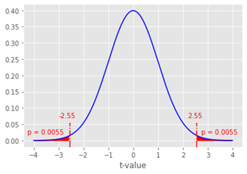
Because our null hypothesis is that the means are equal, we have to look at both tails. Why? Because if the means are not equal one mean could be higher or lower so we need to account for both extremes. If we were only interested in one mean being lower than the other mean we would only need to look at one tail. So, in this case, we need to look at the probabilities where the test statistic is less than -2.55 and more than +2.55 (because the curve is symmetric).
So, now we get to the probabilities or p-values of this occurring. For our example, you can see from the red shaded regions that the p-value for each tail is 0.0055 (or 0.55%). If we add them together, we get 0.0055 + 0.0055 = 0.011. This means there is a 1.1% chance of error in rejecting the null hypothesis. But is this good or bad?
Well, our alpha is 0.05 so we are willing to accept a 5% chance or error. Our p-value is 0.011 which means we have a 1.1% chance of error. Since our chance of error is lower than what we’d be willing to accept, we would REJECT the null hypothesis.
FINAL DECISION
By rejecting the null hypothesis, our decision is that the average order values between the two tests are not equal. Even though the conversion rates were not statistically different, you can now decide if you’d like to implement Test B on account of it having a statistically higher average order value.
EXAMPLE 2 – PRODUCT AND REGIONAL DIFFERENCES
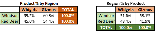
You want to know if the proportion of sales of widgets and gizmos differ in the two regions where they are being sold, Windsor and Red Deer. You want to know at the 95% confidence level. Your unit sales are:

In case you were wondering, the attributes are product and region and the data above is a 2×2 contingency table because we have 2 products (widgets and gizmos) and 2 regions (Windsor and Red Deer).
It’s also important to show this as proportions because visually they look like they’d be different. As a result, we want to test if these differences are indeed statistically different (referred to as statistically significant).
Step 1: State your Hypothesis
For this example, the hypothesis is that the proportion of unit sales for each product in each region is the same. The null hypothesis is that the type of product sold is independent of the region in which it is sold. The alternate hypothesis is that the type of product sold is dependent on the region in which is was sold.
Step 2: Select the Appropriate Statistical Test
In this case we are testing proportions (and each cell value is greater than 5) so we’re going to use the chi-square test. In particular, we have 2 different attributes so we’ll be using the chi-square test for independence.
Step 3: Calculate the test statistic
You could do this the hard way using Excel and a process like the one found here or here; however, you would still need to take your test statistic and determine the p-value against the chi square distribution. So, it’s easier to just use one of the many online calculators like the one found here) as these types of calculators usually include the p-value as well.
After doing the calculations using one of the methods/tools described above for this sample, we get a test statistic of 2.43.
Step 4: Decision Time!
Looking at the chi square distribution graph below and where the test statistic falls, we have to figure out what our p-value is so we can make our decision. The chi-square distribution is not the same as the t-distribution (or normal distribution) but looks like this instead:
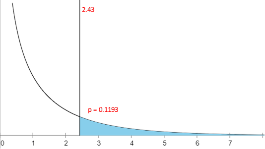
From the graph (or the fact that our tool gave us the test statistic and p-value) we can see that with a test statistic of 2.43 we get a p-value of 0.1193. This means there is an 11.93% chance of error if we reject the null hypothesis. What should we do?
Since our alpha is 0.05, we are willing to accept a 5% chance or error. Our p-value is 0.1193 which means we have an 11.93% chance of error. Since our chance of error is higher than what we’d be willing to accept, we would NOT REJECT the null hypothesis.
Just as an aside and to illustrate the importance of confidence, if you were looking for a 85% confidence, that would be a p-value of 0.15. In this case you would REJECT the null hypothesis so the level of confidence you choose to accept is quite important.
FINAL DECISION
By not rejecting the null hypothesis, our decision is that the products sold are independent of the region in which they are sold with 95% confidence. That means that product sales do not really differ by region with 95% confidence. NOTE: this is not saying that product proportions are the same, it is saying they are about the same by region.
CONCLUSION
In case you actually made it to the end of this post, congratulations! You win the prize of gaining more knowledge about statistical testing (I hope). But, this concludes my 3 part post on some basic statistical principles. I hope you can go forward with some added insight into how to use data and statistics to make better business decisions.